

Dynamic Image Analysis is a perfect method to utilize if not only the particle size of powders is to be determined, but if you also want to ascertain information about their shape. For this purpose the FRITSCH GmbH provides a functional, economically priced instrument, the Particle Sizer ANALYSETTE 28 ImageSizer, which allows dry measurements of free-flowing powders and bulk solids as well as supports measurements with a wet dispersion unit.
Measuring principle
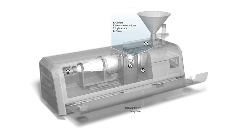
The underlying measuring principle is quickly explained: A directed flow of particles passes in front of a large scale LED flash and the particles are photographed in back light in fast sequences by a digital camera. Therefore, the optical set-up is comparable with transmitted light microscopy, where a high contrast is obtained between the homogeneously lit, light background and the particles shadowing the light. All images are then analysed via software and the corresponding selected data is displayed after the completion of the measurement. More about this later though.
Optical set-up
Let’s dwell on the optical set up though: As with every microscope or common camera, the size of the generated image on the retina or camera sensor depends on the magnification performance of the utilised lens.
For a certain combination of camera and lens, yield from the magnification and the sensor parameters (overall size and pixel size), the limits of this obtainable size range. Inside the ANALYSETTE 28 ImageSizer, runs a 5 mega pixel camera with a 2/3 inch CMOS sensor. The pixel size is 3.45 µm, which in combination with a lens magnification of 0.35 times, results in a lens size of 10 µm per pixel. Now, if for the lower measuring range of the system, images of particles of at least 8 x 8 pixels are required, a lower measuring range of 80 µm is obtained. Through similar deliberations, the upper measuring range of 10 mm is achieved in this combination, i.e. with this combination of camera and lens the particle size range of at least 80 to 10000 µm is covered.
Until now we assumed a constant magnification factor. But this is only possible with regular camera lenses if the distance of the camera to the particle is always identical. If the distance changes the detected particle size is falsified on the same scale. Since in practice it is for the most part impossible to guide the particles exactly on a plane pass the camera, FRITSCH utilizes so-called telecentric lenses here. Unlike with conventional camera lenses, the size of the image generated on the sensor doesn’t depend on the distance between object and camera.
Altogether three different lenses are available for the ANALYSETTE 28 ImageSizer, covering varying measuring ranges. The lenses are changed manually, in a simple process and which can be completed in a short amount of time.
Particle identification

Now how does the instrument recognize the particles? Simply said, the software recognizes dark areas as particles and lighter ones as background. But of course there are numerous gradations between light and dark: The amount of available levels of grey of the camera is 28 = 256 (i.e. the dynamic circumference of the camera is 8 bit). Complete white corresponds to a value of 255, black is 0. In the software, a threshold is specified, which determines whether a pixel belongs to the background or to a particle. For very special sample systems, like for example transparent glass spheres, this threshold can be easily and individually adapted.
Depth of focus
An additional parameter of the optical system comes into play now, the depth of focus. It describes the distance area within which a particle appears sufficiently clear. Basically, the depth of focus of a lens decreases with increasing magnification. Maybe this is familiar from experiences in microscopy where with increasing magnification it becomes increasingly difficult to create a focused image. This causes edges of particles which do not exactly pass the focal plane of the camera, to gradually show a transition from black into white. Based on this transition, the software can now determine which particles are still sufficiently visualized to be considered for evaluation.
Image acquisition speed
Besides the depth of focus, sensor and pixel size, the image acquisition speed - usually indicated as frames per second (fps) - is another not unimportant factor, even though for most applications it does not play a central role. The camera of the ImageSizer obtains up to 75 fps. With such high image rates enormously large volumes of data are generated within a short period of time, demanding the corresponding specifications from the computer hardware in order to handle the measuring task. For example, if a large sample amount for dry measuring is to be measured completely and all images saved, this easily leads only too difficult to manage amounts of data. These can be easily reduced by not permanently saving all images obtained during the measurement or images used for result analysis. However, not every individual particle can be viewed later which is not necessary though during routine measurements.
In practice
At this point, the question arises: How much do I actually have to measure? Like expected, this cannot be generally answered, it strongly depends on the respective sample and the question linked to the measurement. But it can be said, that for most tasks several ten to hundred thousand particles are sufficient, with large particles in the high millimetre range maybe even less. In regards to the needed sample amount it has to be differentiated between a dry or wet measurement.
During a dry measurement, the sample material is continuously fed to the measuring process via a funnel and a vibratory feeder, in which the sample feed speed – how much material per minute is moved – can only be increased within rigid margins: The overlapping of two particle images, which coincidently pass the same visual axis of the camera, should be kept as low as possible. With this procedure, each sample particle is only available once for analysis. In order to avoid an influence of the result from possible segregation tendencies, if possible the entire sample amount which was added to the feed system should be processed, especially for samples with a wide particle size span. With dry measuring, particles of approximately 20 µm up to approximately 20 mm can be measured.
In practice the following has to be considered: Sufficient amounts of material must be used to allow statistically dependable measurements. But not too much in order not to unnecessarily waste time and storage space. To avoid problems with too large analysis amounts, a good sample division should be conducted. Here for example, a FRITSCH Rotary Cone Sample Divider LABORETTE 27 can be utilized, which divides a large overall sample amount into sufficiently small individual samples with identical representative particle size spectrums.
For a wet measurement a good sample division is even more important than for a dry measurement. A closed liquid circuit with a variable volume between 150 ml and 500 ml, is pumped continuously through a measuring cell, the necessary sample amount is therefore clearly less as with a dry measurement. Of course, during the wet measurement the upper measuring limit is determined by the geometry of the measuring cell. With the wet measuring unit of the ANALYSETE 28 ImageSizer particles of approximately 5 µm up to 3 mm can be measured.
Evaluation
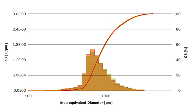
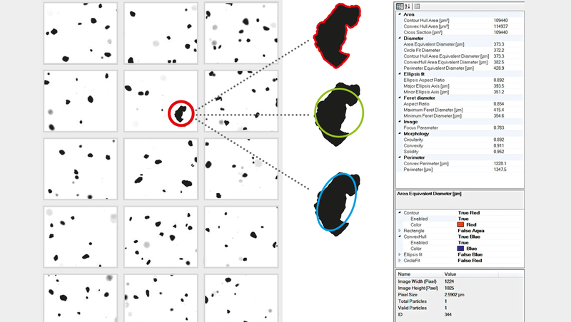
Now what can you do with all these obtained images? Initially of course the particle size can be determined. However the agony of choice starts here already: For example, during static light scattering only one value is given for the particle diameter, of course an imaging system offers different possibilities to define the diameter of a mostly irregularly shaped particle. Examples for this can be the area equivalent diameter (the diameter of a sphere, whose cross section has the same area as the evaluated particle), the diameter calculated from the particle circumference, or the so called Feret diameter, where two parallel lines on opposing sides of a particle are arranged so that they touch the particle, but don’t intersect the particle edge.
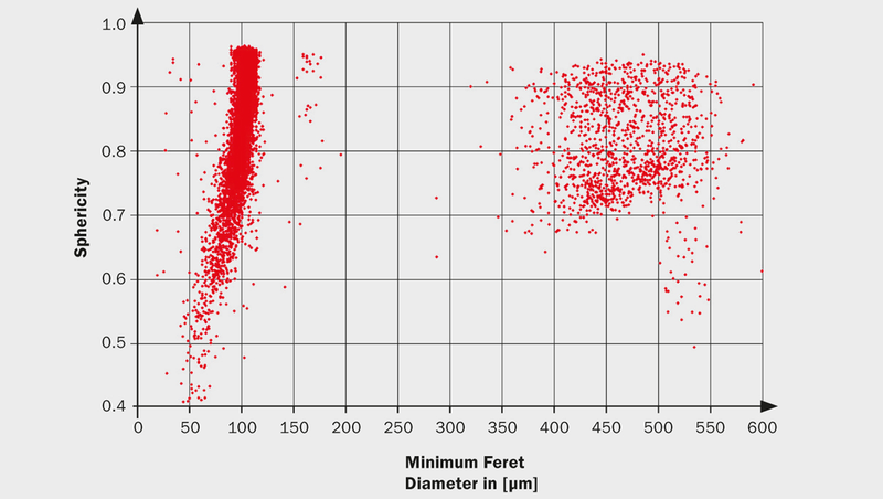
A decisive advantage of the Dynamic Image Analysis lies of course in the possibility that besides the basic determination of the diameter, also information about the geometry of the particles can be obtained. As one of the simplest shape parameters, the aspect ratio shall be mentioned here, which is yielded as the quotient from minimum to maximum Feret diameter.
With the ImageSizing-Software ISS of the ANALYSETTE 28 it is possible to quickly and simply generate distributions and correlations in any random combination of particle sizes: Whether this is only a simple size distribution or the connection between the particle size and the aspect ratio. In a Cloud presentation such correlations can be graphically displayed especially simple and fast. Each analysed particle is shown here as a point and its coordinates in the Cloud depend on the values of each selected parameter. Especially with new sample materials and the analysis of problematic cases, one feature of the cloud is especially helpful: By clicking on the point of a selected particle, the corresponding image opens.
-
Download the FRITSCH-report as PDF file

FRITSCH GmbH - Milling and Sizing
55743 Idar-Oberstein

